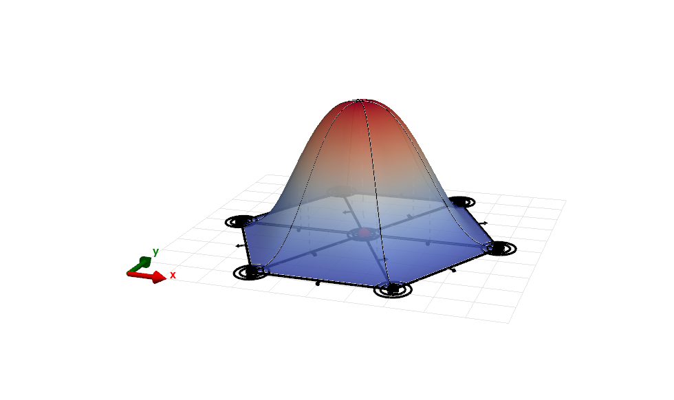
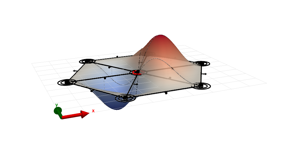
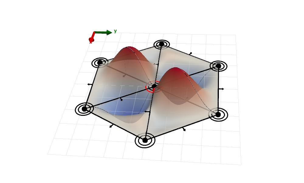
Higher Order Finite Elements

This is an exploration of polynomial functions defined on simplicial finite elements. I will not give much background, the goal here is to visualize trial functions for more complex elements, which are hard to find. I use the diagram style of Brenner & Scott to show the degrees of freedom - a dot for a value constrained node, a ring/arrow for a gradient constrained node, a double ring/double arrow for a hessian constrained node, and a lone arrow to specify a lone gradient component.

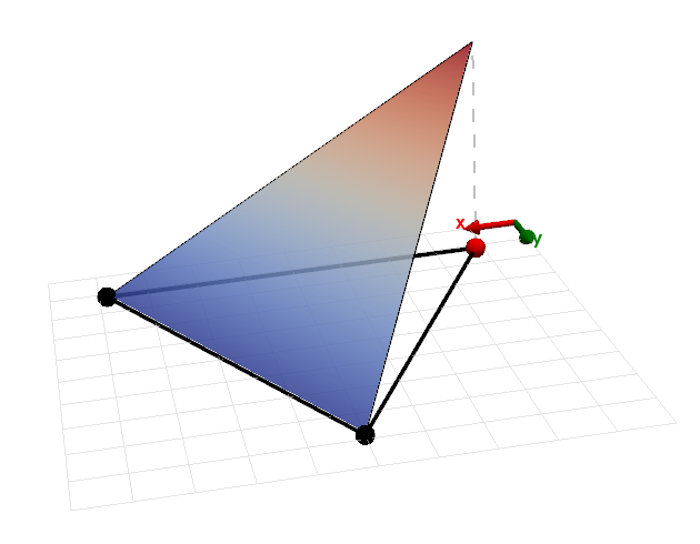
For most FEM solves, linear elements suffice. Consider the prototypical Poisson equation in 2D, \(\frac{\partial^2 u}{\partial x^2} + \frac{\partial^2 u}{\partial y^2} + f = 0\). The usual setup is we seek a function \(\tilde{u}=\sum_{i \in I_s}{c_i \phi_i}\), where \(I_s\) is the set of degrees of freedom (DOFs), and the set of \(\phi_i\) form the trial function space \(V\), that minimizes the residual \(R(\tilde{u})=\Delta \tilde{u} + f\). Using, say, the Galerkin method, we minimize \(R\) within \(V\) by requiring \(\langle \phi_i, R \rangle =0\) for all \(i\). Using integration by parts magic, this involves computing \(\langle \phi_i', \phi_j' \rangle\) for all \(i\) and \(j\). That is, we only require \(\phi_i\) to be in the Sobolev space \(W^{1, 2}\). Presumably we want \(\tilde{u}\), so each \(\phi_i\) to be continuous as well. The simplest such construction is the linear element with 3 ‘value’ DOFs, on at each vertex of the triangle. This is shown for a single DOF of a single triangle below, as well as for a DOF and its one-ring. The DOF in question is shown in red.

Its reasonable to suspect that we may want a C1 solution in some cases. This may be strictly required, e.g. when using the collocation method for a first order PDE. Maybe our application specifies that we need a C1 solution. In 1D this is doable with a cubic hermite elements, but in 2D this is not so simple a task. Clearly any polynomial is C1 inside an element. To check if a trial function for a DOF is C1, we must show that it has zero gradient on the boundary of its nonzero domain, and that it has a continuous gradient on the boundary between triangles in its nonzero domain. Suppose we try a cubic polynomial surface. This has 10 coefficients. For this to be C1 with its neighbors, the gradient on each boundary must be unique along the boundary. Since each gradient term is quadratic, there must be 4 constraints. Playing with the DOFs you will see the issue - as we increase the polynomial degree to get more DOFs to constrain the boundary, we require more constraints on the boundary since the gradient itself is of higher degree. It turns out the best we can do is a quintic polynomial - the Argyris element. We constrain the value, gradient, and hessian at each vertex. We also add a normal gradient DOF at the midpoint of each edge. In this way, the gradient has 5 constraints (the gradient and hessian and the endpoints and the normal gradient at the midpoint), defining a unique quartic. Below are the Argyris DOF functions shown for the one-ring of a corner DOF (\(\phi\), \(\partial_x \phi\), \(\partial_{xy} \phi\), in order), and the normal gradient DOF at the edge boundary. Visually, this thing is C1.